Introduction to Tensors in Pytorch #2

This is the second part of the "Introduction to Tensors in PyTorch". If you missed the first part, read it from here and come back later on this post.

So far I have discussed the basics of tensors in the previous post related to defining, reshaping and casting the datatypes. But they are not limited to such operations, in fact, you can perform arithmetic calculations, matrix multiplication and other statistical functions like mean, and etc.

In this post, you will learn the following

• Indexing and Slicing of Tensors
• Arithmetic Operations on Tensors
• Basic Functions on the Tensors
• Operations on 2D Tensors

So let's begin...

Indexing and Slicing of Tensors

PyTorch was created to provide pythonic ways to deal with tensors. Like normal array slicing or indexing, you can also perform such operations on the tensors. The values in return will also be a tensor. The dimension of the tensors in indexing will be one less than the actual dimension.

import torch

t1 = torch.tensor([1, 2, 3, 4])
print(t1[0])

"""
Output:
tensor(1)
"""

Since the original tensor was of 1-D, the value would be of course a 0-D tensor. So to if you have a 2-D tensor, and are doing using only one index, you will get a 1-D tensor

import torch

t2 = torch.tensor([[1, 2, 3, 4], [5, 6, 7, 8]])
print(t2[0])

"""
Output:
tensor([1, 2, 3, 4])
"""

NOTE: If you want to get the raw python list of 1+ D tensors, you can use Tensor.tolist() method

Like a normal list, you can also update the tensor value by simply accessing the index. For example

t1[2] = 100
print(t1)

"""
Output:
tensor([1, 2, 100, 4])
"""

NOTE For your sake, PyTorch returns a new tensor object whenever you perform slicing on the original tensor. But it will overwrite the original tensor when you will change the value of the tensor at a particular index. Read More

In the 2-D tensor, the slicing can be done both on rows and columns or either of them. The first part before the comma (,) means rows and the second part means column. So it will look like Tensor[ROW, COL]

t3 = torch.randint(0, 10, size=(3, 3))
print(t3)

# Get all the elements from 2nd row
print(t3[1, :])

# Get first element from 2nd row and 1st column 
print(t3[1, 0])

# Get all the rows after 2nd (including) and all the elements from 
# these rows' columns first 2 element
print(t3[1:, :2])

"""
Output:
tensor([[6, 6, 7],
        [8, 6, 5],
        [3, 4, 4]])
tensor([8, 6, 5])
tensor(8)
tensor([[8, 6],
        [3, 4]])
"""

Arithmetic Operations on Tensors

The very basic operations on tensors are vector additions and subtractions. Visit the link in case you want to study the maths behind these vector operations

Suppose you have two tensors \(u\) and \(v\) defined as

u = torch.tensor([1.0, 2.0])
v = torch.tensor([3.0, 4.0])

print(u)
print(v)

"""
Output:
tensor([1., 2.])
tensor([3., 4.])
"""

Then the vector operations addition and subtraction respectively

print(u + v)
print(u - v)

"""
Output
tensor([4., 6.])
tensor([-2., -2.])
"""

Scalar operations are also supported. For example, taking \(5\) as our scalar quantity

ws = torch.tensor(5)
print(ws)

"""
Output:
tensor(5)
"""

The operations addition, subtraction, multiplication and division are shown respectively

print(u + v + ws)
print(u + v - ws)
print(u + v * ws)
print(u + (v / ws))

"""
Output:
tensor([ 9., 11.])
tensor([-1.,  1.])
tensor([16., 22.])
tensor([1.6000, 2.8000])
"""

In PyTorch, there is no need of creating a 0-D tensor to perform scalar operations you can simply use the scalar value and perform the action. For example,

print(v * 5)

"""
Output:
tensor([15., 20.])
"""

The cross-product is fairly short and easy, by using the * symbol. But to perform dot product, you should use torch.dot(vector1, vector2) or Tensor.dot(vector2). The dot product will return a 0-D tensor as defined in maths

print(u * v)
print(torch.dot(u, v))
print(u.dot(v))

"""
Output:
tensor([3., 8.])
tensor(11.)
tensor(11.)
"""

NOTE While performing cross-product or dot-product, dimensions of both the tensors should be equal, otherwise you will get RuntimeError

Basic Functions on the Tensors

Torch tensors provide a plethora of functions that you can apply to the tensors for the desired results. The first one of all is Tensor.mean()

x = torch.tensor([1, 2, 3, 4, 5], dtype=torch.float32)
print(x)
print(x.mean())

"""
Output:
tensor([1., 2., 3., 4., 5.])
tensor(3.)
"""

NOTE Since the mean of a tensor will be a floating tensor, you can find the mean of floating tensor only otherwise you will get RuntimeError

Finding maximum or minimum value in the tensor can be done by using Tensor.max() and Tensor.min() respectively

print(x.max())
print(x.min())

"""
Output:
tensor(5.)
tensor(1.)
"""

You can also apply a function to a tensor element-wise. Suppose you have a tensor containing various values of pi and you want to apply the sin and cos function on it. You can use torch.sin(tensor) and torch.cos(tensor)

import numpy as np

x = torch.tensor([0, np.pi / 2, np.pi])
print(x)
print(torch.sin(x))
print(torch.cos(x))

"""
Output:
tensor([0.0000, 1.5708, 3.1416])
tensor([ 0.0000e+00,  1.0000e+00, -8.7423e-08])
tensor([ 1.0000e+00, -4.3711e-08, -1.0000e+00])
"""

Sometimes you will have to get an evenly spaced list of numbers between a range, you can use torch.linspace(start, end, [step]). Let's make it more interactive by plotting the \(\sin (- \pi ) \) to \( \sin ( \pi ) \) and \( \cos (- \pi ) \) to \( \cos ( \pi ) \).

pi = torch.linspace(-np.pi/2, np.pi/2, steps=1000)
print(pi[:5])  # lower bound
print(pi[-5:]) # upper bound

sined = torch.sin(pi)
cosed = torch.cos(pi)
print(sined[0:5])
print(cosed[0:5])

"""
Output:
tensor([-1.5708, -1.5677, -1.5645, -1.5614, -1.5582])
tensor([1.5582, 1.5614, 1.5645, 1.5677, 1.5708])
tensor([-1.0000, -1.0000, -1.0000, -1.0000, -0.9999])
tensor([-4.3711e-08,  3.1447e-03,  6.2894e-03,  9.4340e-03,  1.2579e-02])
"""

Now let's import matplotlib and plot both the graphs for sined and cosed tensors.

import matplotlib.pyplot as plt

plt.plot(sined, label="sined")
plt.plot(cosed, label="cosed")
plt.legend()
plt.show()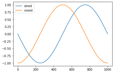

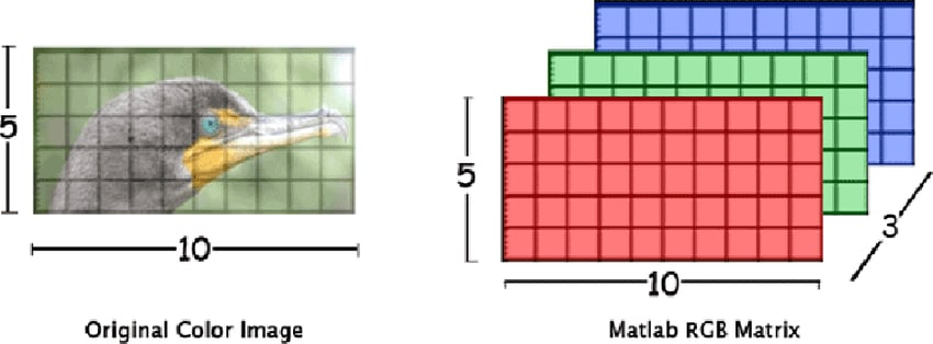
Operations on 2D Tensors

The greyscale images are the best example of 2D tensors. Each pixel which you see as \( width * height \) are the \( cols * rows \) for the matrix.

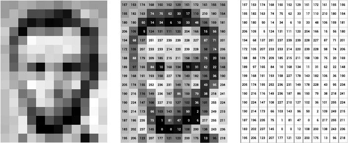
In the above images, it is demonstrated how a binary image can be represented in a matrix. In the case of a grayscale image, the value of each element of the matrix would be in the range of \( 0 - 255 \).

Creating a random 2D tensor using the torch.rand(*size) method. This is a general method, you can create a random tensor of any dimension using this method. The Tensor.numel() method used above returns the total number of elements in the tensor.

t2 = torch.rand((3, 3))
print(t2)

# dimension of matrix is also called rank of matrix
print(t2.ndim)
print(t2.shape)
print(t2.numel())

"""
Output:
tensor([[0.0376, 0.4297, 0.2987],
        [0.8009, 0.1815, 0.5538],
        [0.2482, 0.7099, 0.3132]])
2
torch.Size([3, 3])
9
"""

To perform the matrix multiplication you can use either of them: Tensor.matmul(tensor2), torch.matmul(tensor1, tensor2), Tensor.mm(tensor2) or torch.mm(tensor1, tensor2)

x = torch.rand((3, 4))
y = torch.rand((4, 3))
print(x)
print(y)

print(x.matmul(y))
print(torch.mm(x, y))

"""
Output:
tensor([[0.6413, 0.1338, 0.5066, 0.1618],
        [0.3807, 0.8555, 0.2187, 0.5024],
        [0.2771, 0.6381, 0.5671, 0.6934]])
tensor([[0.0263, 0.9461, 0.6314],
        [0.9180, 0.1586, 0.2589],
        [0.3363, 0.4529, 0.9433],
        [0.6760, 0.8877, 0.1171]])
tensor([[0.4195, 1.0009, 0.9363],
        [1.2086, 1.0409, 0.7270],
        [1.2525, 1.2358, 0.9563]])
tensor([[0.4195, 1.0009, 0.9363],
        [1.2086, 1.0409, 0.7270],
        [1.2525, 1.2358, 0.9563]])
"""